CFD Simulation Methods for High-Lift Aircraft Configurations (Part 3 of 3)
In this series we will highlight contributions to the 4th AIAA High Lift Prediction Workshop using a variety of CFD simulation techniques. The full series consists of three parts: Part Iprovides essential background motivation for carrying out this study. Part II will detail our modeling strategy and discuss the computational fluid dynamics approach. Part III will showcase the results and how they are useful in enhancing our understanding of flow behavior in high-lift configurations.
PART III – Sensitivity Results and Recommendations
In PART II of the series, we discussed details about the tools and techniques used for modeling an aircraft using CFD. In this final part of the series, we present the results obtained from our suite of fluid dynamics simulations of a modeled HL-CRM aircraft in high-lift configuration using Flow360.
Effect of Grid Refinement
We begin by examining the behavior of lift coefficient (CL) versus the freesteam angle of attack (⍺) as we change the resolution of the ANSA type grids. The results are presented in Figure 1.
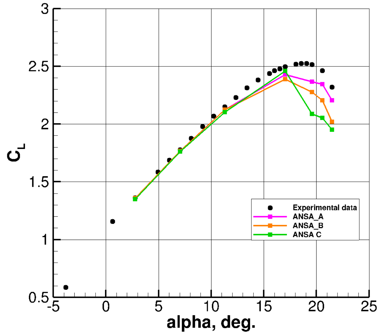
Figure 1: Comparison of lift coefficient for simulations with different ANSA grid resolutions.
The results show excellent agreement in the linear region (smaller ⍺). Near CL max, fairly good agreement is obtained for the ANSA A mesh (68 million nodes) when compared to experimental data. However, mesh refinement unfortunately leads to poorer predictions at high lift. The finer grids predict sharper stall with lower CL values at each angle of attack in the non-linear region (higher ⍺). This suggests that the coarser grids benefit from a cancellation of errors, for this particular quantity at least, which is not entirely unexpected.
It is very illuminating to analyze the distribution of skin friction (Cf) on the model wing surface. We observe that for lower ⍺ all the grids show very similar Cf profiles (not shown), which results in similar integrated loads on the wing. However, at larger ⍺ in the non-linear regime, the skin friction behavior is very different in some areas of the wing. Regions where Cf approaches zero implies local boundary layer separation.
As shown in Figure 2, skin friction contours vary significantly for the inboard wing region. The coarsest mesh, ANSA A, has only a small streamwise region of near-zero Cf adjacent to the fuselage. Alternatively, ANSA C results display a very large region of separation downstream of the nacelle. This enlarged flow separation helps explain the smaller lift coefficients found at higher grid resolutions. We can further comment that the flow separation at higher resolution is due to different resolutions of the grid capturing the different vortical structures coming from the slat, slat-junctions, pylon, and chine. In the outer parts of the wing where such vortical structures are not present, a high degree of agreement among different grid sizes can be seen.

Figure 2: Skin friction distributions at ⍺=19.57° for different levels of ANSA grid refinement
Effect of Grid Element Types
Next, we examine the effect of using different grid element topologies, with consideration also for grid resolutions, built with Pointwise. Three topologies of the grid elements were used: tetrahedral only (Tet), tetrahedral with prism layers (Tet-Prism), and fully mixed (Tet-Prism-Hex-Pyramid). In these cases, we fix the angle of attack to 7.05°.
In Figure 3, we show the convergence of CL with respect to grid refinement for the three topologies. We can see that CL values for all types of grid elements are comparable with each other, with a more refined grid in each case generally leading to a better agreement with the experimental value. However, we should be cautious when generalizing these results since calculations were performed for only a single angle of attack.
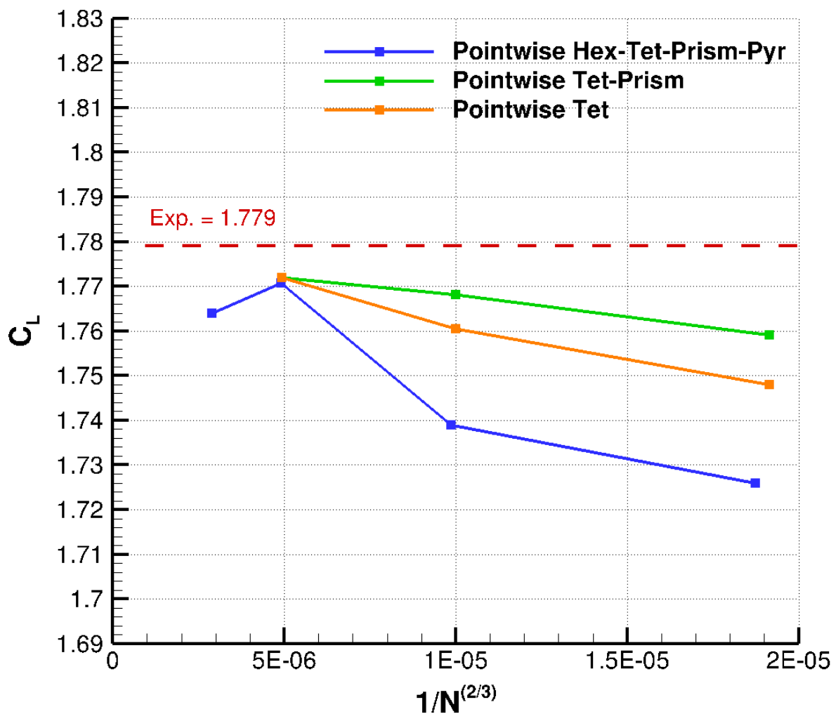
Figure 3: Grid convergence of CL at α = 7.05° using different Pointwise grid topologies.
Here, N is the number of nodes and the x-axis displays more refined grids at left.
Comparing ANSA with PW Grids
Let us now compare the ANSA C grid and Pointwise D (Hex-dominated) grids. These grids have a similar node counts of around 200 million, but were generated by two different meshing softwares and methodologies (see PART II). Once again, we compare the lift coefficient of two grids at different angles of attack in Figure 4. It should be noted here that these simulations were ‘warm’ started. That is, each subsequent α is restarted from the previous α simulation, rather than from freestream initialization.
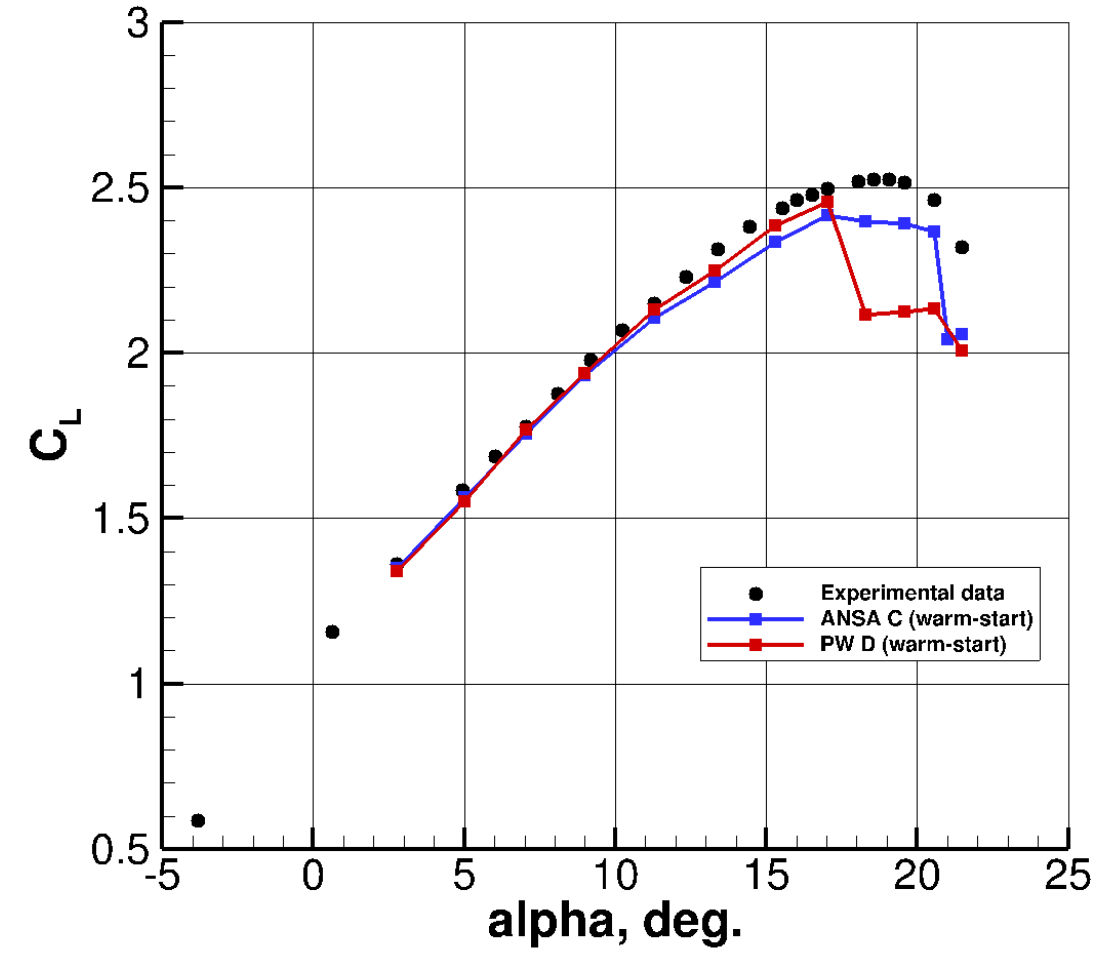
Figure 4: Lift coefficient behavior at different angles of attack and with different grid types.
The comparison indicates similar results in the linear region of the lift curve. As α is spooled-up further (in between α = 11.29° and α = 17.05°) the Pointwise grid leads to a slightly higher lift at a given angle of attack. In the non-linear region, the Pointwise grid exhibits a much sharper stall, indicated by a sharp drop in lift coefficient. The ANSA grid, in contrast, predicts a shallow stall, with only a minor underprediction in CL compared to experimental data. Both grids lead to similar results at the highest examined α = 21.47° with an underpredicted lift when compared to experimental data.
In order to investigate the difference in behavior at higher α, we present the Cf distribution across the wing in Figure 5. At α = 19.57°, Cf patterns in the wing tip region differ somewhat. A significant difference between the two grids is observed over the wing in the nacelle region, where the flow separates strongly past the nacelle for the Pointwise grid, with only a minor reduction in Cf seen for the ANSA grid. Both grids show similar Cf distributions at the root of the wing.
It is clear that the main reason for the sharp drop in lift coefficient for the Pointwise grid simulations is due to the large separation past the nacelle, which is not present in the ANSA grid results. However, at the highest angle of attack of 21.47°, the flow in the wing root is completely separated for both ANSA and Pointwise grids, leading to similar wing lift behavior. The unfortunate overall conclusion is that high-lift configurations can be sensitive to local mesh resolution and methodology.
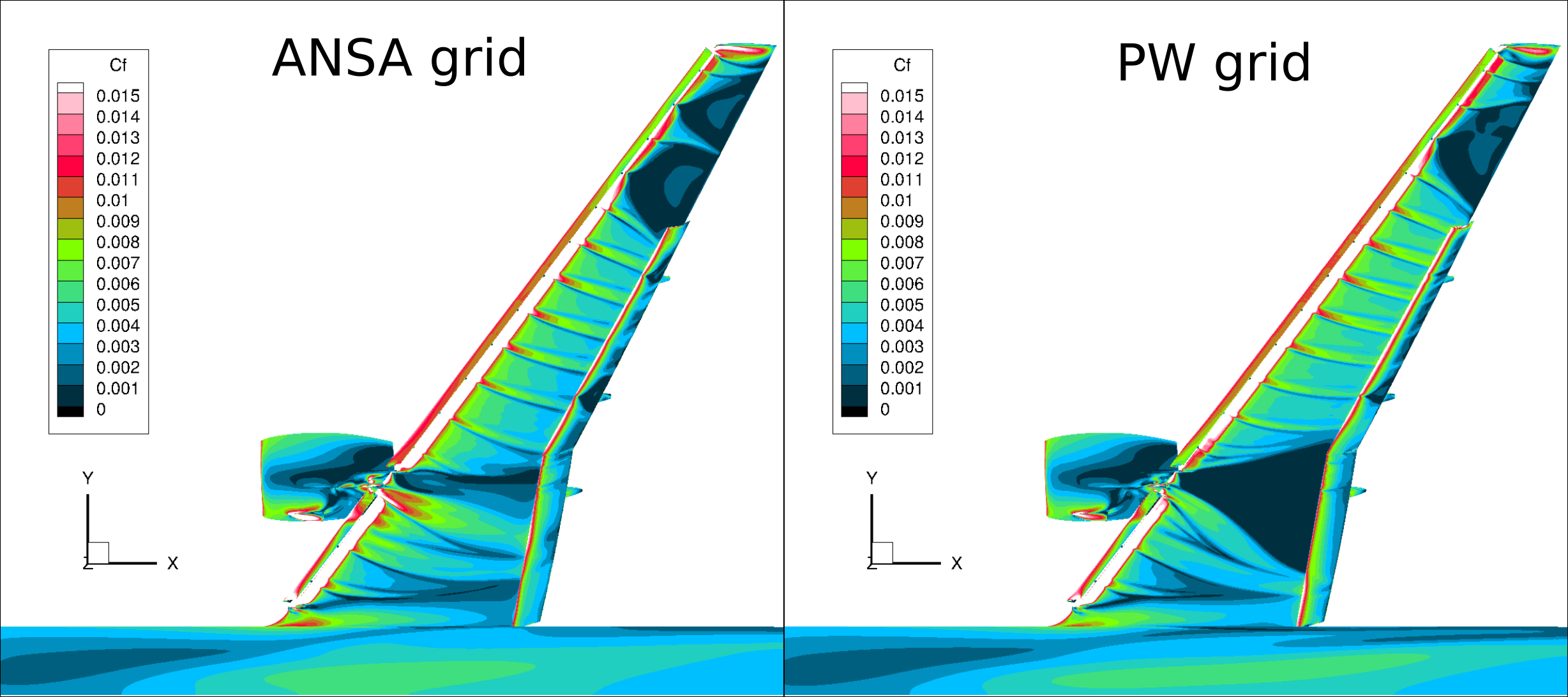
Figure 5: Skin friction behavior for ANSA grid and PW grid at α = 19.57°.
Effect of Cold- vs Warm-Starts
We now examine how the simulations behave when started with different initial conditions. As we mentioned earlier, cold-start solutions are performed by initializing the simulation from freestream conditions, which means that the flow field develops completely during the convergence of the simulation. Warm-started simulations initialize the flow field from the previous angle of attack solution and update the farfield boundary with the current angle of attack. Warm-start simulations can reduce computational cost because the flow field is already well established.
Furthermore, we also carried out two different warm-start approaches, starting from different angles of attack, α = 2.78° and α = 17.05°. For the warm-start from α = 17.05°, all lower angles of attack (including α = 17.05° ) used cold-start solutions, and the warm-start cases were progressively started from the prior α. The simulations in these cases were performed on the ANSA C grid (about 200 million nodes).
We compare the lift coefficient for different approaches in Figure 6. The results show that the starting condition has a large impact on the final result of a simulation. The cold-started solutions show an early stall compared to experiment. Warm-starting the solution leads to much closer agreement with experimental data.
The difference in behavior between the cold- and warm-started cases is made evident in Figure 7 where flow separates downstream of the nacelle in the cold-started case while no substantial flow separation is seen for the warm-started cases.
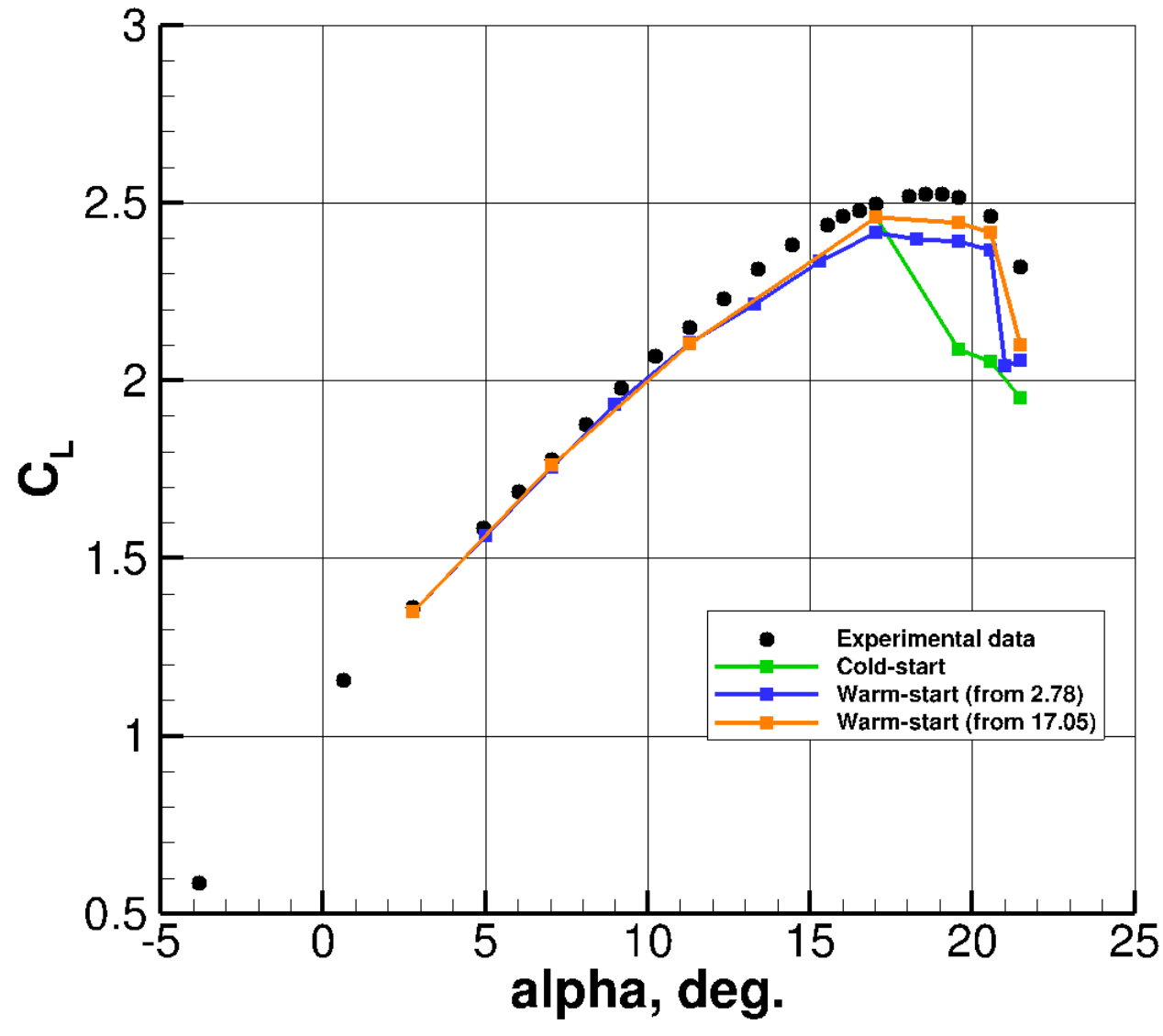
Figure 6: Comparison of CL for cold and warm started simulations.

Figure 7: Skin friction distributions using warm-started and cold-started simulations.
The analysis of warm- and cold-started solutions shows that initializing a simulation from the previous angle of attack can be favorable in RANS predictions for highly separated flows. The cold-started simulations can develop unexpected separation during flow field convergence, which tends to remain in the solution until the simulation is stopped. Here, the unfortunate conclusion (which is relevant to RANS solvers) is that current technology does not ensure unique solutions.
Comparison with DES
Based on our study, we believe that a warm started ANSA C grid with the SA turbulence model can be considered a “best practice” when it comes to agreement with the experimental data.
We now present a comparison of this best practice case with a delayed Detached Eddy Simulation (DES) which is unsteady and scale resolving, and therefore much more computationally expensive. We perform two DES simulations, one at CL max and one past CL max, α = 19.57° and 21.47°, respectively. The DES simulations were also run on the ANSA C grid. Furthermore, the DES simulations were performed for 40 convective time units (CTUs) for α = 19.57° and 80 CTUs for α = 21.47°. The last 20 CTU’s were used for solution averaging for α = 19.57° and 40 CTUs for α = 21.47° – this helps to capture the longer time scales associated with large eddies and massive separation.
The results are shown in Figure 8, with the error bars for the DES simulations corresponding to splitting the signal into 10 samples in order to gauge the adequacy of the averaging time interval. It is clear from the figure that significant improvements for high-lift predictions can be obtained by moving to DES simulations.
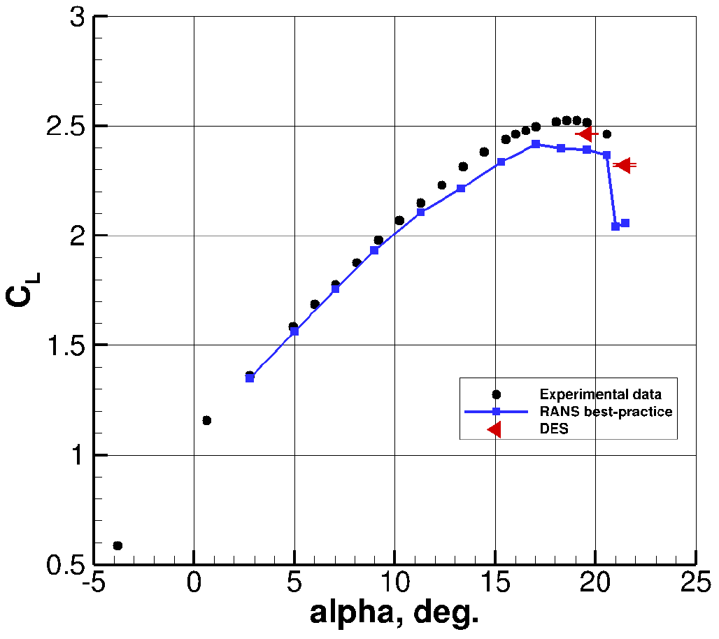
Figure 8: Comparison of CL for best-practice RANS and DES cases.
The Cf distributions presented in FIgure 9 show the superiority of DES for high-lift predictions over the RANS-based approach. At both examined angles of attack, the DES simulations capture the slat bracket wakes more accurately with significantly reduced separated flow regions near the wing tip.
Further inboard, the DES simulation does not predict any significant drop in Cf in the flow past the nacelle. The wing root region also appears to lead to large differences between the steady RANS and DES predictions. The DES simulation at α = 19.57° shows a minor separation region at the root extending upstream from the trailing edge, which is not present in the RANS solution. The prediction at α = 21.47° for the DES simulation is significantly improved with reduced separation present over the root region of the wing compared to the RANS solution.
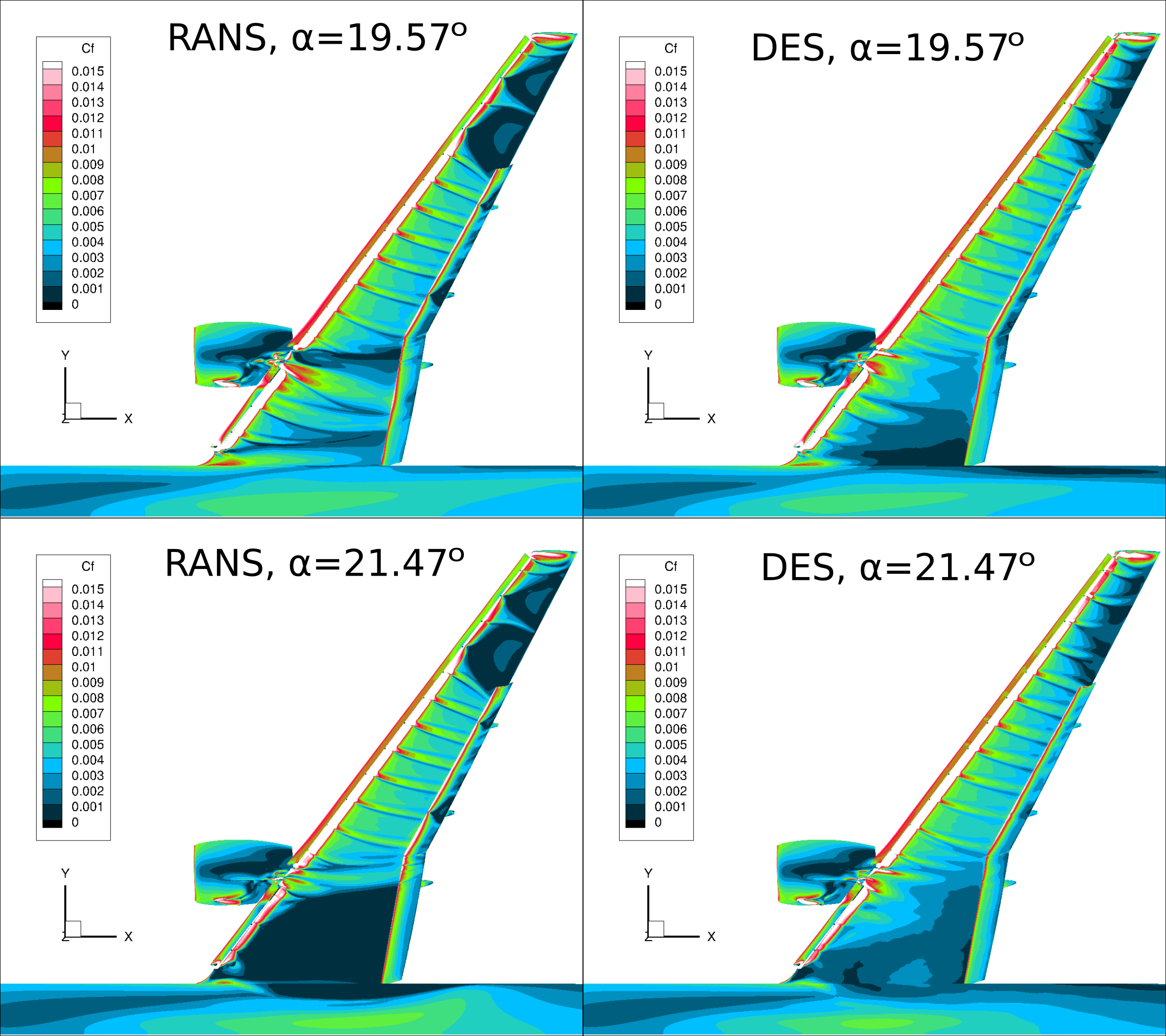
Figure 9: Comparison of Cf for RANS and DES simulations at α = 19.57° and α = 21.47°.
Conclusions
After a broad examination of the modeling sensitivities for RANS-based solutions, we provide a few recommendations:
- RANS-based approaches show a high grid sensitivity and therefore require intelligent grid design aimed at resolving all of the complex interactions present in the flow field, whether through user iteration on the mesh resolution or through mesh adaptation.
- The current results indicate the existence of multiple solutions when using RANS, with the best-practice results obtained when initializing the flow field from the previous angle of attack (warm-start).
Besides the recommendations for best RANS practices, however, further analysis of the RANS results along with DES simulations highlighted the shortcomings of RANS-based solutions and the need for scale-resolving simulations for accurate high-lift predictions. The DES simulations are able to capture the flow physics of high-lift flows with a higher degree of accuracy, but at a significant increase in computational costs. It is conceivable, however, that with constantly growing computational power and the need for more accurate CFD predictions, scale-resolving simulations may become more prominent in future High Lift Prediction Workshops and elsewhere.
This concludes the series of articles. If you’d like to learn more about CFD simulations, how to optimize them, or how to reduce your simulation time from weeks or days to hours or minutes, stop by our website at Flexcompute.com or follow us on LinkedIn.
For the expanded version of the paper this content is derived from, see An Analysis of Modeling Sensitivity Effects for High Lift Predictions using the Flow360 CFD Solver.


