Multimode Photonics Design Made Easy
By Lucas GabrielliDesigning multimode devices can be a complex task. In this session, we present the tools available in Tidy3D that facilitate this process and enable precise control over mode excitation, decomposition, and tracking in dielectric waveguides. In a real device, we show the importance of modal decomposition analysis when designing multimode photonics.
Session 2: Multimode Photonics Design Made Easy
In this workshop, we characterize and compare two designs of multimode waveguide bends. The first design is the usual circular bend, which, as we'll see, leads to strong mode mixing in the waveguide. The second option is based on the works by Xiaohui Jiang, Hao Wu, and Daoxin Dai, "Low-loss and low-crosstalk multimode waveguide bend on silicon," Opt. Express 26, 17680-17689 (2018), doi: 10.1364/OE.26.017680 [1]. It uses the Euler Spiral to generate a bend with continuous curvature, which mitigates much of the mode mixing even at a small radius [2].
Analysis of multimode devices depends on the precise evaluation of the transmission in the modes of interest and couplings to undesired ones, characterizing inter-mode cross-talk or mode mixing.
The steps we'll take are the following:
- define the device geometry;
- investigate the modes supported by our multimode waveguide;
- configure our simulation to excite the desired mode and perform modal decomposition at the output;
- compare both designs in terms of transmission and mode mixing.
We start by importing all required modules for this notebook.
import numpy as np
import matplotlib.pyplot as plt
from scipy.special import fresnel
import gdstk

import tidy3d as td
from tidy3d import web
from tidy3d.plugins.mode import ModeSolver
from tidy3d.plugins.mode import web as ms_web
Bend Geometry
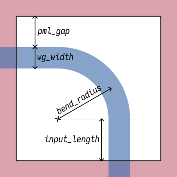
The simulation setup for the bend geometry is straightforward. The required dimensions are illustrated below and defined in the following code block.
It is important to bring a couple of aspects to attention:
- The input and output waveguides stretch straight into the PML regions at a normal angle with the PML interface. If not, the PML should be substituted by an absorbing layer because the fields would most likely diverge in the PML.
- There is a section of straight waveguide before the bend in both input and output regions, which allows us to place the source and monitors far enough from the bend for the fields to accommodate.
- We leave a lateral gap between the waveguide and the PML for the evanescent tails of the waveguide modes. This is also true in the out-of-plane (z) dimension, which is not shown in the figure.
# Free-space wavelength (in um) and frequency (in Hz)
wavelengths = np.linspace(1.45, 1.65, 11)
freqs = td.C_0 / wavelengths
freq0 = freqs[freqs.size // 2]
fwidth = freqs.max() - freqs.min()

# Permittivity of waveguide and substrate
mat_wg = td.material_library["cSi"]["Li1993_293K"]
mat_sub = td.material_library["SiO2"]["Horiba"]

# Lengths are defined in μm
wg_height = 0.22
wg_width = 1.0
input_length = 0.5
bend_radius = 4.0  # bend radius
pml_gap = 1.0  # lateral distance between waveguide and the PML

# Simulation domain size and total run time
sim_length = input_length + bend_radius + wg_width / 2 + pml_gap
sim_size = (sim_length, sim_length, 2)
run_time = 10 / fwidth

# Grid specification
grid_spec = td.GridSpec.auto(min_steps_per_wvl=20, wavelength=wavelengths.min())
The geometry is defined with the help of the gdstk module to draw the waveguide. The Euler bend is created with two helper functions.
The bends' exact derivation is beyond this workshop's scope, but it is pretty straightforward from the definition of the Euler spiral.
The waveguide_geometry function generates the whole waveguide geometry and takes the type of bend as a parameter, which can be set to "circular" or "euler".
Note that the straight sections of the waveguide are created with an added sim_length dimension to ensure full overlap with the PML.
def euler_bend_helper(rmin, n):
    """Euler bend helper function."""
    l = 0.25 * np.pi * rmin
    b = np.sqrt(rmin * l * np.pi / 2)
    u = np.linspace(0, 1, n)
    z = u * l / b
    y, x = fresnel(z)
    y *= b
    x *= b
    xe = np.hstack((-y, x[-2::-1] - x[-1] - y[-1]))
    ye = np.hstack((x, -y[-2::-1] + y[-1] + x[-1]))
    return xe, ye


def euler_bend(r: float, max_step: float) -> tuple[np.ndarray, np.ndarray]:
    """Calculate the x, y coordinates for a 90° euler bend.

    Args:
        r: Effective bend radius.
        max_step: Maximal distance between calculated points.

    Returns:
        (x, y): Coordinate arrays.
    """
    x, y = euler_bend_helper(1, 2)
    rmin = r * 2 ** 0.5 / np.sqrt(x[-1] ** 2 + y[-1] ** 2)
    n = max(2, 1 + int(np.ceil(0.25 * np.pi * rmin / max_step)))
    return euler_bend_helper(rmin, n)


def waveguide_geometry(bend_type: str) -> td.Geometry:
    path = gdstk.RobustPath((input_length + bend_radius, -sim_length), wg_width)
    path.vertical(sim_length + input_length, relative=True)
    if bend_type == "euler":
        x, y = euler_bend(bend_radius, 0.2)
        x = x[1:] + input_length + bend_radius
        y = y[1:] + input_length
        for xy in zip(x, y):
            path.segment(xy)
    elif bend_type == "circular":
        path.turn(bend_radius, np.pi / 2)
    path.horizontal(-sim_length - input_length, relative=True)

    # Create a gdstk cell that can be loaded by tidy3d
    cell = gdstk.Cell("Bend").add(path)

    # Return the waveguide geometry
    return td.Geometry.from_gds(
        cell,
        axis=2,
        slab_bounds=(-0.5 * wg_height, 0.5 * wg_height),
        gds_layer=0,
        gds_dtype=0,
    )
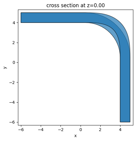
We can compare the geometries of the 2 bend types by plotting them together with some transparency:
geom_circ = waveguide_geometry("circular")
ax = geom_circ.plot(z=0, alpha=0.7)

geom_euler = waveguide_geometry("euler")
_ = geom_euler.plot(z=0, ax=ax, alpha=0.7)

# _ = ax.set_xlim(0, None)
# _ = ax.set_ylim(0, None)
Defining the Simulation
We use the previous function to parametrize our simulation with the bend type.
It is usually a good idea to have our simulation defined in a function so that we can easily perform parameter sweeps and optimizations later on.
We are interested in evaluating the bend with respect to the fundamental waveguide mode.
We can excite a specific mode in a waveguide with a ModeSource.
Mode sources use Tidy3D's Mode Solver to compute the modes supported by the waveguide cross-section where they are defined.
We can monitor the power transmitted through the waveguide cross-section at the output in 2 manners:
-
A
FluxMonitorcan be used to compute the total integrated flux through the cross-section. This measurement will not differentiate between modes; it will compute the total power going through the monitor plane (including scattered light, which is why it is important to have some distance from the end of the curve). -
Similar to a
ModeSource, aModeMonitorwill also use the internal mode solver to calculate the modes supported by the output waveguide cross-section and decompose the radiation into the calculated mode base. This calculation also differentiates forward- and backward-propagating modes, which is handy for reflection calculations.
We will use both types of monitor to illustrate their uses and differences.
Furthermore, we also add a FieldMonitor to inspect the distribution of the fields (in the frequency domain) over the simulation domain in the xy plane.
def simulation(bend_type: str, num_modes: int) -> td.Simulation:
    # Waveguide
    waveguide = td.Structure(
        geometry=waveguide_geometry(bend_type),
        medium=mat_wg,
    )

    mode_spec = td.ModeSpec(num_modes=num_modes)

    # Source
    mode_src = td.ModeSource(
        center=(input_length + bend_radius, 0.2 * input_length, 0),
        size=(2 * pml_gap, 0, sim_size[2]),
        source_time=td.GaussianPulse(freq0=freq0, fwidth=fwidth),
        mode_spec=mode_spec,
        mode_index=0,
        direction="+",
        num_freqs=7,
    )

    # Modal monitor at a range of frequencies
    mode_mnt = td.ModeMonitor(
        center=(0.2 * input_length, input_length + bend_radius, 0),
        size=(0, 2 * pml_gap, sim_size[2]),
        freqs=freqs.tolist(),
        mode_spec=mode_spec,
        name="mode",
    )

    # Flux monitor
    flux_mnt = td.FluxMonitor(
        center=mode_mnt.center, size=mode_mnt.size, freqs=mode_mnt.freqs, name="flux"
    )

    # Frequency-domain field monitor at central frequency
    field_mnt = td.FieldMonitor(
        center=(0, 0, 0), size=(td.inf, td.inf, 0), freqs=[freq0], name="field"
    )

    sim = td.Simulation(
        center=(sim_length / 2, sim_length / 2, 0),
        size=sim_size,
        grid_spec=grid_spec,
        structures=[waveguide],
        medium=mat_sub,
        sources=[mode_src],
        monitors=[field_mnt, mode_mnt, flux_mnt],
        run_time=run_time,
        boundary_spec=td.BoundarySpec.all_sides(boundary=td.PML()),
    )
    return sim
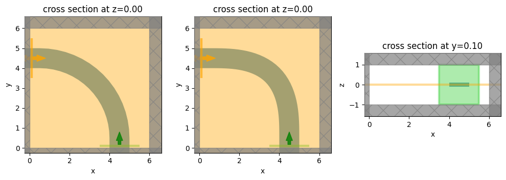
We make sure our domain looks correct before running the simulation by plotting a couple of cross-sections.
fig, ax = plt.subplots(1, 3, figsize=(10, 4), tight_layout=True)

circ_sim = simulation("circular", 6)
_ = circ_sim.plot(z=0, ax=ax[0])

euler_sim = simulation("euler", 6)
_ = euler_sim.plot(z=0, ax=ax[1])

_ = circ_sim.plot(y=0.2 * input_length, ax=ax[2])
Inspecting the Waveguide Modes
Before running the simulation, we can inspect the modes from our waveguides to ensure our sources and monitors are properly set and make any design modifications we see fit (such as changing the waveguide cross-section to support more or fewer modes).
We can use the Mode Solver plugin by directly creating a ModeSolver object.
In our case, because we already have mode sources and monitors defined in a simulation, we can use them directly:
source = circ_sim.sources[0]

mode_solver = ModeSolver(
    simulation=circ_sim,
    plane=source.bounding_box,
    mode_spec=source.mode_spec,
    direction=source.direction,
    freqs=[freq0],
)
It is possible to run the mode solver locally or using the backend solver. The local solver can be faster for small jobs because there's no overhead of submitting the specifications and downloading the results, but the remote solver has support for subpixel smoothing, which improves the accuracy of the solutions, especially when the waveguide cross-section geometry doesn't align to the underlying grid.
# Uncomment this line to use the local mode solver
# mode_data = mode_solver.solve()

# Here, we use the remote mode solver
mode_data = ms_web.run(mode_solver, task_name="Multimode bend modes")

mode_data.to_dataframe()
18:07:45 UTC Mode solver created with
             task_id='fdve-c15a78a6-3f73-426b-a160-7a9c6dda9f94',
             solver_id='mo-697fc21d-ddde-4a5e-91b3-35540a2b0f5b'.
18:07:46 UTC Mode solver status: queued
18:07:58 UTC Mode solver status: running
18:08:11 UTC Mode solver status: success
| wavelength | n eff | k eff | loss (dB/cm) | TE (Ex) fraction | wg TE fraction | wg TM fraction | mode area | ||
|---|---|---|---|---|---|---|---|---|---|
| f | mode_index | ||||||||
| 1.934145e+14 | 0 | 1.55 | 2.741531 | 0.000025 | 8.850609 | 0.998469 | 0.929991 | 0.805580 | 0.235038 |
| 1 | 1.55 | 2.416970 | 0.000041 | 14.381480 | 0.989456 | 0.740152 | 0.836074 | 0.333873 | |
| 2 | 1.55 | 1.971824 | 0.000204 | 71.774441 | 0.028022 | 0.634709 | 0.941026 | 0.476068 | |
| 3 | 1.55 | 1.821291 | 0.000103 | 36.311228 | 0.928711 | 0.575276 | 0.893321 | 0.485969 | |
| 4 | 1.55 | 1.677453 | 0.000240 | 84.578156 | 0.124583 | 0.741909 | 0.747073 | 0.618127 | |
| 5 | 1.55 | 1.433924 | 0.000200 | 70.361769 | 0.518302 | 0.927000 | 0.987226 | 2.395468 |
num_modes = mode_solver.mode_spec.num_modes

fig, ax = plt.subplots(num_modes, 3, figsize=(12, 2.5 * num_modes), tight_layout=True)

for mode_index in range(num_modes):
    mode_solver.plot_field("S", "abs^2", f=freq0, mode_index=mode_index, robust=False, ax=ax[mode_index, 0])
    mode_solver.plot_field("Ex", "real", f=freq0, mode_index=mode_index, robust=False, ax=ax[mode_index, 1])
    mode_solver.plot_field("Ez", "real", f=freq0, mode_index=mode_index, robust=False, ax=ax[mode_index, 2])
    ax[mode_index, 0].set_title(f"n_eff[{mode_index}] = {mode_data.n_eff.sel(f=freq0, mode_index=mode_index):.2f}")
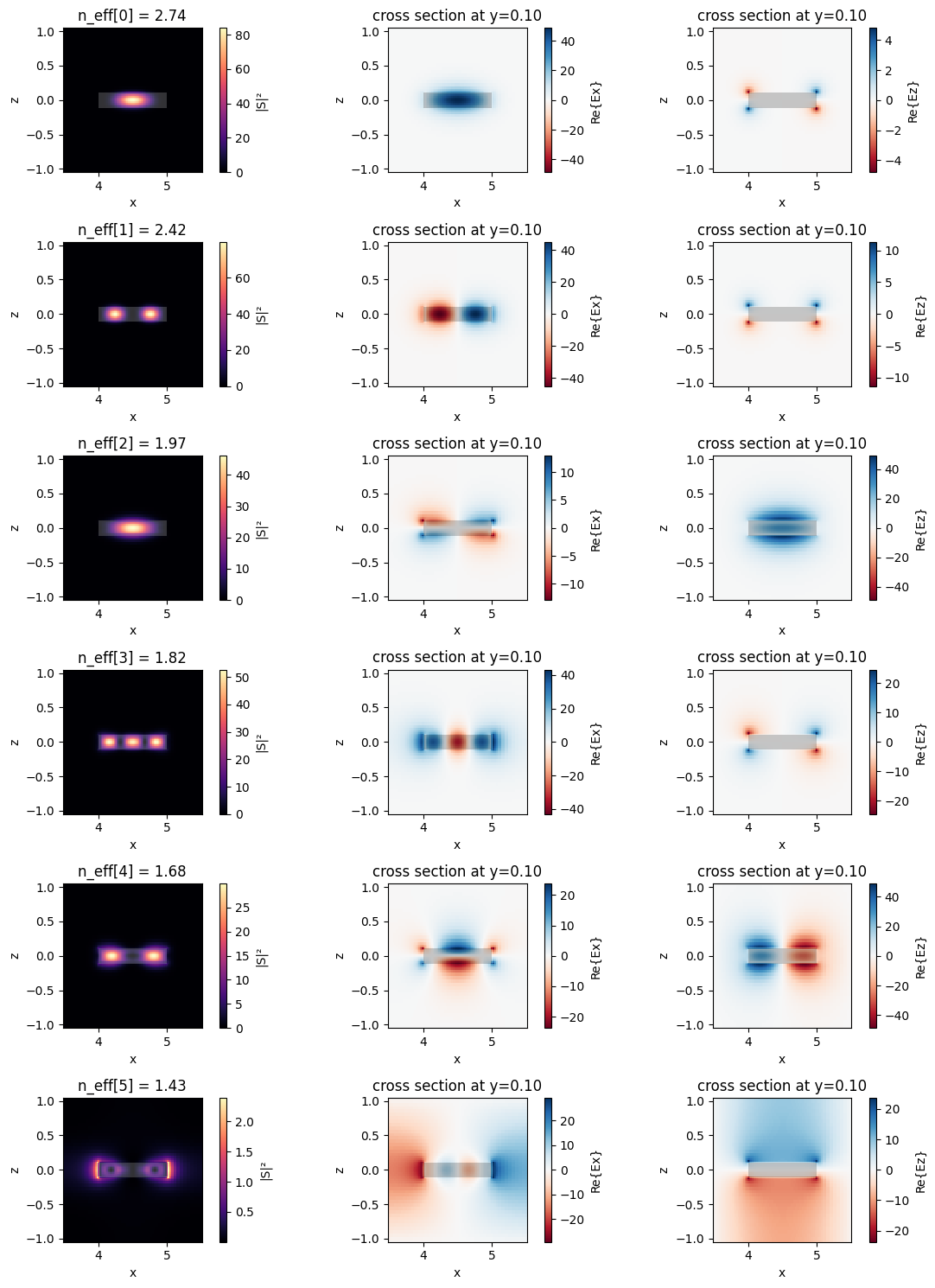
We see that the waveguide supports 5 modes. The last one is below the light line of the SiO₂ cladding, which means that it is a "domain mode" defined by the boundary conditions of the domain. That's the reason why we should always make sure the mode sources and monitors have cross-sections large enough to accommodate the evanescent tails of all modes of interest.
We could do the same investigation for the monitor modes, but they will be identical to these because the waveguide has the same cross-section.
Further Mode Investigation
The mode solver can also give information about the group index and dispersion by changing the mode specification. Note that group index and dispersion calculations are more sensitive to the grid resolution, so a greater mesh refinement should be used when calculating them.
mode_spec2 = mode_solver.mode_spec.updated_copy(group_index_step=True)
mode_solver2 = mode_solver.updated_copy(mode_spec=mode_spec2)
mode_data2 = ms_web.run(mode_solver2, task_name="Multimode bend modes 2")
mode_data2.to_dataframe()
18:08:17 UTC Mode solver created with
             task_id='fdve-bf85d184-2a43-40af-a77d-732cc4d989bd',
             solver_id='mo-17d54bb8-8803-4500-9ec2-730956f838af'.
18:08:18 UTC Mode solver status: queued
18:08:29 UTC Mode solver status: running
18:08:41 UTC Mode solver status: success
| wavelength | n eff | k eff | loss (dB/cm) | TE (Ex) fraction | wg TE fraction | wg TM fraction | mode area | group index | ||
|---|---|---|---|---|---|---|---|---|---|---|
| f | mode_index | |||||||||
| 1.934145e+14 | 0 | 1.55 | 2.741531 | 0.000025 | 8.850609 | 0.998469 | 0.929991 | 0.805580 | 0.235038 | 3.819993 |
| 1 | 1.55 | 2.416970 | 0.000041 | 14.381480 | 0.989456 | 0.740152 | 0.836074 | 0.333873 | 4.267146 | |
| 2 | 1.55 | 1.971824 | 0.000204 | 71.774441 | 0.028022 | 0.634709 | 0.941026 | 0.476068 | 4.028410 | |
| 3 | 1.55 | 1.821291 | 0.000103 | 36.311228 | 0.928711 | 0.575276 | 0.893321 | 0.485969 | 4.866588 | |
| 4 | 1.55 | 1.677453 | 0.000240 | 84.578156 | 0.124583 | 0.741909 | 0.747073 | 0.618127 | 4.051053 | |
| 5 | 1.55 | 1.433924 | 0.000200 | 70.361769 | 0.518302 | 0.927000 | 0.987226 | 2.395468 | 1.937476 |
Simulation Run
We run the simulation as usual through the web API, wait for it to finish, and download the results.
Note: Make sure to create the "data" folder if it doesn't exist!
job = web.Job(simulation=simulation("circular", 5), task_name="Circular Bend", verbose=True)
circ_data = job.run(path="data/circular_bend.hdf5")
             Created task 'Circular Bend' with task_id
             'fdve-3793845f-8ed4-4bc8-a8be-d509b1bacb23' and task_type 'FDTD'.
             View task using web UI at
             'https://tidy3d.simulation.cloud/workbench?taskId=fdve-3793845f-8ed
             4-4bc8-a8be-d509b1bacb23'.
status = success
18:08:42 UTC loading simulation from data/circular_bend.hdf5
Let's first examine the in-plane fields recorded by the frequency monitor. We can already see how the source emits all of its power in the desired direction and waveguide mode.
_ = circ_data.plot_field("field", "Hz", "real", f=freq0, robust=False)
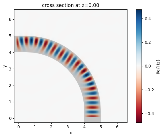
We note that in Tidy3D, the fields recorded by frequency monitors (and thus also mode monitors) are automatically normalized by the power amplitude spectrum of the source (for multiple sources, the user can select which source to use for the normalization). Furthermore, mode sources are normalized to inject exactly 1W of power at the central frequency.
Knowing that, we can check the total bend transmission from the flux monitor:
# Flux monitor (total power through the cross-section)
flux = circ_data["flux"].flux
print("Flux at central frequency: ", flux.sel(f=freq0).values)
Flux at central frequency: -0.9972616
We can also use the mode amplitudes recorded in the mode monitor to reveal the decomposition of the radiated power into forward- and backward-propagating modes.
In this case, we're only interested in the modes in the "-" direction (propagating towards -y in our simulation).
# Field amplitude coefficients for each mode in the -y direction
mode_amps = circ_data["mode"]
coeffs = mode_amps.amps.sel(direction="-")

fig, ax = plt.subplots(1, figsize=(6, 4), tight_layout=True)

ax.plot(wavelengths, np.abs(flux), "--")
ax.plot(wavelengths, np.abs(coeffs.values) ** 2)
ax.set_title("Circular bend transmission")
ax.set_xlabel("Wavelength (um)")
ax.set_ylabel("Power (W)")

_ = ax.legend(["Flux"] + [f"Mode {i}" for i in range(num_modes)])
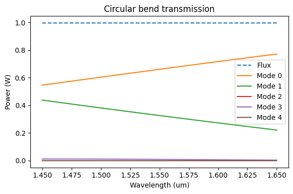
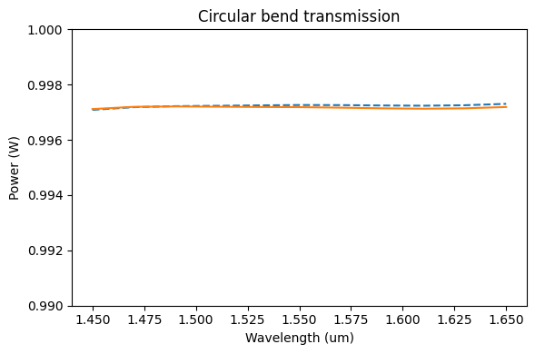
We can compare the total power measured by the flux monitor and the sum over all modes in the decomposition. In this case, because all modes are accounted for and we're not measuring scattered power in the flux monitor, they match very closely.
# Field amplitude coefficients for each mode in the -y direction
mode_amps = circ_data["mode"]
coeffs = mode_amps.amps.sel(direction="-")

fig, ax = plt.subplots(1, figsize=(6, 4), tight_layout=True)

ax.plot(wavelengths, np.abs(flux), "--", label="Flux")
ax.plot(wavelengths, (np.abs(coeffs) ** 2).sum("mode_index").values, label="Sum of modes")
ax.set_title("Circular bend transmission")
ax.set_xlabel("Wavelength (um)")
ax.set_ylabel("Power (W)")
_ = ax.set_ylim(0.99, 1)
Now, we solve the Euler bend to compare.
job = web.Job(simulation=simulation("euler", 5), task_name="Euler Bend", verbose=True)
euler_data = job.run(path="data/euler_bend.hdf5")
18:08:44 UTC Created task 'Euler Bend' with task_id
             'fdve-9761ac5b-9425-4a89-b7ae-4c27ff008749' and task_type 'FDTD'.
             View task using web UI at
             'https://tidy3d.simulation.cloud/workbench?taskId=fdve-9761ac5b-942
             5-4a89-b7ae-4c27ff008749'.
status = success
loading simulation from data/euler_bend.hdf5
_ = euler_data.plot_field("field", "Hz", "real", f=freq0, robust=False)
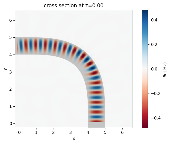
We can already see less mode mixing from the field profile in the frequency domain, but we still want to quantify it by looking at the mode decomposition at the output.
# Forward and backward power amplitude coefficients
mode_amps = euler_data["mode"]
coeffs = mode_amps.amps.sel(direction="-")

fig, ax = plt.subplots(1, figsize=(6, 4), tight_layout=True)

ax.plot(wavelengths, np.abs(flux), "--")
ax.plot(wavelengths, np.abs(coeffs.values) ** 2)
ax.set_title("Euler bend transmission")
ax.set_xlabel("Wavelength (um)")
ax.set_ylabel("Power (W)")

_ = ax.legend(["Flux"] + [f"Mode {i}" for i in range(num_modes)])
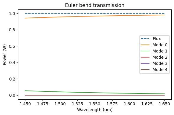
The difference is clear! The continuous curvature variation in the Euler bend helps to keep most of the input power in the fundamental mode even on a bend with a (effective) radius of only 4 µm.
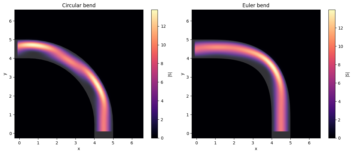
We can look at the Poynting vector on both curves to see the process by which mode coupling happens:
fig, ax = plt.subplots(1, 2, figsize=(12, 5), tight_layout=True)

circ_data.plot_field("field", "S", "abs", f=freq0, robust=False, ax=ax[0])
ax[0].set_title("Circular bend")

euler_data.plot_field("field", "S", "abs", f=freq0, robust=False, ax=ax[1])
_ = ax[1].set_title("Euler bend")
Activity Description
Modify the simulation setup presented in the session notebook to perform the following additional analyses.
-
Compute and compare the mode transmission through the Euler and the Circular bends for the first 3 waveguide modes. Check if the Euler bend is equally effective for higher-order modes.
-
Re-parametrize the simulation by radius of curvature and plot a curve of total transmission efficiency by effective radius for the wavelengths of 1.45, 1.55, and 1.65 μm. Use the fundamental mode to excite the waveguide and consider the effective radius values of 1, 1.5, 2, and 3 µm. Include the first 6 waveguide modes in the calculation of the total transmission efficiency. Then, compare the results obtained by the Euler and Circular bends.
You can develop this example using the Tidy3D Python notebook or the Graphical User Interface (GUI) web-based environments. See the FDTD Learning Center for Python and GUI tutorials.
References
[1] Xiaohui Jiang, Hao Wu, and Daoxin Dai, "Low-loss and low-crosstalk multimode waveguide bend on silicon," Opt. Express 26, 17680-17689 (2018), doi: 10.1364/OE.26.017680.
[2] Florian Vogelbacher, Stefan Nevlacsil, Martin Sagmeister, Jochen Kraft, Karl Unterrainer, and Rainer Hainberger, "Analysis of silicon nitride partial Euler waveguide bends," Opt. Express 27, 31394-31406 (2019), doi: 10.1364/OE.27.031394.