Designing Filters and Reflectors with Bragg Gratings
By Tom ChenBragg gratings are periodic structures used in various optical systems. The periodicity allows Bragg gratings to reflect specific wavelengths of light while transmitting others. The key principle behind their operation is the Bragg’s condition. This section will introduce the Bragg condition and use Tidy3D to model a distributed Bragg reflector and cavity. Then, we will apply the same principle to integrated photonics and demonstrate the design of silicon waveguide Bragg gratings.
Session 3: Designing Filters and Reflectors
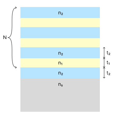
A distributed Bragg reflector (DBR) is a multilayer structure consisting of alternating layers of high refractive index and low refractive index. When the thickness of each layer is close to a quarter of the medium wavelength, nearly perfect reflection occurs due to constructive interference of the reflected waves at each layer. DBR is commonly used at optical and UV wavelengths because metallic reflectors have a high loss at high frequencies. Besides free space optics, similar concepts have also been applied to integrated photonics and fiber optics. Furthermore, high-Q cavities based on DBR structures are widely popular in lasers, filters, and sensors.
Sometimes, for instance, in the coating of Fabry-Perot interferometers, the DBR starts and ends with the higher refractive index thin film. In this case, when considering quarter-wave thin films at normal light incidence, the reflectance $R_{N+1}$ is given by [1]
$$ R_{N+1} = \left(\frac{n_{s}n_{0}(n_{1})^{2N} - n_{2}^{(2N+2)}}{n_{s}n_{0}(n_{1})^{2N} + n_{2}^{(2N+2)}}\right)^{2}, $$where $N$ is the number of layer pairs, $n_{0}$ is the air refractive index, $n_{s}$ is the substrate refractive index, $n_{1}$ is the lower refractive index, and $n_{2}$ is the higher refractive index. The layer thicknesses are calculated by $n_{1}t_{1} = n_{2}t_{2} = \lambda/4$ ($\lambda$ is the light wavelength).
Activity 1
In this activity, we will walk you through the design of a DBR thin film reflector, calculate its reflectance spectrum, and compare its value at the center wavelength with the one obtained by the analytical expression. Please see the Distributed Bragg reflector and cavity example and use it as a reference.
We will also demonstrate how to make frequency-domain animation and time-domain animation.
Step 1
Start by including the necessary libraries below.
import numpy as np
import matplotlib.pyplot as plt

import tidy3d as td
import tidy3d.web as web
Step 2
Define the mediums you will need to build the DBR. Consider $n_{0} = 1$, $n_{s} = 1.52$, $n_{1} = 1.35$, and $n_{2} = 2.30$.
n_0 = 1.00  # air refractive index.
n_1 = 1.35  # lower refractive index.
n_2 = 2.30  # higher refractive index.
n_s = 1.52  # substrate refractive index.

medium_0 = td.Medium(permittivity=n_0**2)
medium_1 = td.Medium(permittivity=n_1**2)
medium_2 = td.Medium(permittivity=n_2**2)
medium_s = td.Medium(permittivity=n_s**2)
Step 3
Calculate the layer thicknesses $t_{1}$ and $t_{2}$ considering $\lambda = 0.546$ $\mu m$, and create a DBR structure with $N = 4$ pairs plus a starting high index thin film.
lda0 = 0.546  # light wavelength.
N = 4  # number of layer pairs.
t_1 = lda0 / (4 * n_1)  # lower refractive index thin film thickness.
t_2 = lda0 / (4 * n_2)  # higher refractive index thin film thickness.
z_0 = 0  # z coordinate of the layer (modify as needed).
inf_eff = 10  # effective infinity in this model.
run_time = 1e-13  # simulation run time

DBR = []  # holder for the DBR structure.

# build the substrate structure.
sub = td.Structure(
    geometry=td.Box.from_bounds(rmin=(-inf_eff, -inf_eff, -inf_eff), rmax=(inf_eff, inf_eff, 0)),
    medium=medium_s,
)
DBR.append(sub)

# build the first layer.
layer_1 = td.Structure(
    geometry=td.Box.from_bounds(rmin=(-inf_eff, -inf_eff, 0), rmax=(inf_eff, inf_eff, t_2)),
    medium=medium_2,
)
DBR.append(layer_1)
z_0 = t_2

# include the N pairs of layers alternatively.
for i in range(2 * N):
    if i % 2 == 0:
        DBR.append(
            td.Structure(
                geometry=td.Box.from_bounds(
                    rmin=(-inf_eff, -inf_eff, z_0),
                    rmax=(inf_eff, inf_eff, z_0 + t_1),
                ),
                medium=medium_1,
            )
        )
        z_0 = z_0 + t_1
    else:
        DBR.append(
            td.Structure(
                geometry=td.Box.from_bounds(
                    rmin=(-inf_eff, -inf_eff, z_0),
                    rmax=(inf_eff, inf_eff, z_0 + t_2),
                ),
                medium=medium_2,
            )
        )
        z_0 = z_0 + t_2
Step 4
Above the DBR structure, include a plane wave excitation source normally incident to the top thin film surface.
thickness = t_2 + N * (t_1 + t_2)  # MODIFY this value to include the DBR multilayer thickness.
src_z_pos = thickness + 3 * lda0  # source position.
freq0 = td.C_0 / lda0  # source frequency.
fwidth = 0.5 * freq0  # width of the frequency distribution.
freqs = freq0 * np.linspace(0.5, 1.5, 1001)  # frequency range of interest.

plane_wave = td.PlaneWave(
    source_time=td.GaussianPulse(freq0=freq0, fwidth=fwidth),
    size=(td.inf, td.inf, 0),
    center=(0, 0, src_z_pos),
    direction="-",
    pol_angle=0,
)
Step 5
Include a flux monitor above the plane wave source to measure the reflectance and a field monitor at the xz plane to calculate the electromagnetic field distribution. In addition, a field time monitor should be included to create an animation of pulse propagation.
# Flux monitor to measure the reflectance.
flux_monitor = td.FluxMonitor(
    center=(0, 0, src_z_pos + lda0 / 4),
    size=(td.inf, td.inf, 0),
    freqs=freqs,
    name="R",
)

# Field monitor to visualize the EM field distribution.
field_xz = td.FieldMonitor(
    center=(0, 0, 0),
    size=(td.inf, 0, td.inf),
    freqs=[freq0],
    name="field_xz",
    interval_space=(10, 1, 1),
)

# Field time monitor to record animation frames
movie_monitor = td.FieldTimeMonitor(
    center=(0, 0, 0),
    size=(td.inf, 0, td.inf),
    fields=["Ex"],
    start=0,
    stop=run_time / 2,
    interval=5,
    interval_space=(100, 1, 3),
    name="movie",
)
Step 6
Build the FDTD simulation. First, define the simulation domain size. As we have translational symmetry in the xy plane, we could set the dimensions in the x- and y-directions to zero and run a 1D simulation. However, as we want to see the Fourier-transformed field distribution, we will set a 2D simulation. The dimension in the z-direction is calculated based on the DBR multilayer thickness. To avoid evanescent waves within the absorbing boundaries (which can result in divergences), you should include a minimum space of $\lambda/2$ between the top and bottom DBR layers and the edges of the simulation domain in the z-direction.
Set the simulation grid to AutoGrid with 60 steps per wavelength. Include periodic boundary conditions in the x- and y-directions, as well as PML boundaries in the z-directions, to absorb the outgoing waves completely. Set the simulation run time to 1 ps and the shutoff to 1e-7 to increase simulation accuracy.
Lx = 1  # Domain size in x-direction.
Ly = 0  # Domain size in y-direction.
Lz = 10 * thickness  # Domain size in z-direction.

sim = td.Simulation(
    size=(Lx, Ly, Lz),  # simulation domain size.
    center=(0, 0, thickness / 2),
    grid_spec=td.GridSpec.auto(min_steps_per_wvl=60, wavelength=lda0),
    structures=DBR,
    sources=[plane_wave],
    monitors=[flux_monitor, field_xz, movie_monitor],
    run_time=run_time,
    boundary_spec=td.BoundarySpec(
        x=td.Boundary.periodic(), y=td.Boundary.periodic(), z=td.Boundary.pml()
    ),  # pml is applied in the z-direction.
    shutoff=1e-7,
)  # early shutoff level is decreased to 1e-7 to increase the simulation accuracy.
Step 7
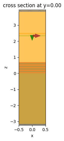
Check the simulation setup to verify if all the components are in their correct places and run the simulation.
# visulize the simulation setup.
ax = sim.plot(y=0)
ax.set_aspect(0.6)
# run the simulation.
sim_data = web.run(sim, task_name="DBR", path="data/simulation.hdf5", verbose=True)
15:39:22 -03 Created task 'DBR' with task_id
             'fdve-0bc42663-d6c6-4b14-9d67-c49e741ea767' and task_type 'FDTD'.
             View task using web UI at
             'https://tidy3d.simulation.cloud/workbench?taskId=fdve-0bc42663-d6c
             6-4b14-9d67-c49e741ea767'.
15:39:25 -03 status = queued
15:39:29 -03 status = preprocess
15:39:35 -03 Maximum FlexCredit cost: 0.025. Use 'web.real_cost(task_id)' to get
             the billed FlexCredit cost after a simulation run.
starting up solver
running solver
             To cancel the simulation, use 'web.abort(task_id)' or
             'web.delete(task_id)' or abort/delete the task in the web UI.
             Terminating the Python script will not stop the job running on the
             cloud.
15:39:43 -03 early shutoff detected at 76%, exiting.
15:39:44 -03 status = postprocess
15:39:49 -03 status = success
             View simulation result at
             'https://tidy3d.simulation.cloud/workbench?taskId=fdve-0bc42663-d6c
             6-4b14-9d67-c49e741ea767'.
15:39:53 -03 loading simulation from data/simulation.hdf5
Step 8
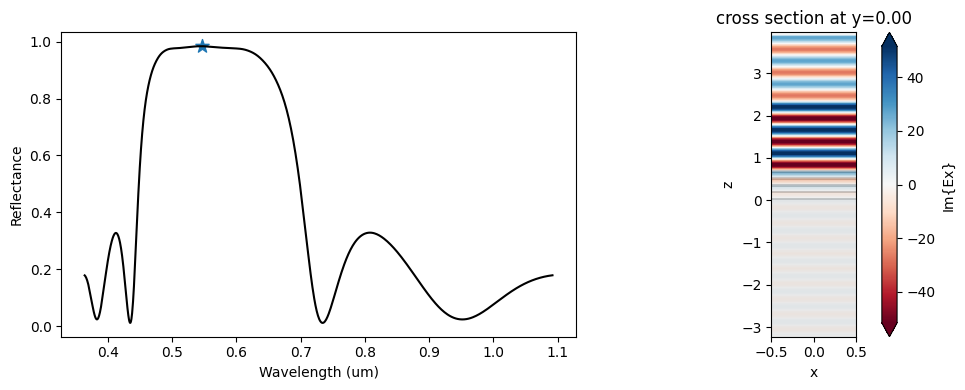
Verify the simulation results, calculate the DBR reflectance using the analytical expression in the introduction, and compare the results.
R = sim_data["R"].flux  # extracting reflectance data from the flux monitor.
R_c = (
    ((n_s * n_0 * n_1 ** (2 * N)) - (n_2 ** (2 * N + 2)))
    / ((n_s * n_0 * n_1 ** (2 * N)) + (n_2 ** (2 * N + 2)))
) ** 2
wl_range = td.C_0 / freqs  # wavelength range.

f, (ax1, ax2) = plt.subplots(1, 2, figsize=(10, 4), tight_layout=True)
ax1.plot(wl_range, R, "-k")
ax1.scatter(lda0, R_c, marker="*", s=100)
ax1.set_xlabel("Wavelength (um)")
ax1.set_ylabel("Reflectance")

sim_data.plot_field("field_xz", "Ex", val="imag", ax=ax2)
ax2.set_aspect(0.5)
plt.show()
Create frequency domain animation.
import matplotlib.animation as animation
from IPython.display import HTML

frames = 50  # number of frames

fig, ax = plt.subplots()

def animate(i):
    phase = -2 * np.pi * i / frames
    sim_data["field_xz"].apply_phase(phase).Ex.real.plot(
        x="x", y="z", ax=ax, vmin=-60, vmax=60, add_colorbar=False, cmap="RdBu"
    )
    ax.set_aspect(0.7)

# create animation
ani = animation.FuncAnimation(fig, animate, frames=frames)
plt.close()

# display the animation
HTML(ani.to_jshtml())
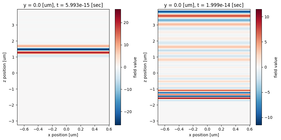
Inspect the field at certain time instances, namely 6 fs and 20 fs.
fig, ax = plt.subplots(1, 2, figsize=(10, 5), tight_layout=True)

sim_data["movie"].Ex.sel(t=6e-15, method="nearest").plot(x="x", y="z", ax=ax[0])

sim_data["movie"].Ex.sel(t=2e-14, method="nearest").plot(x="x", y="z", ax=ax[1])
plt.show()
Create time domain animation.
t_end = sim_data["movie"].Ex.coords["t"][-1]  # end time of the animation

fig, ax = plt.subplots()

def animate(i):
    t = t_end * i / frames  # time at each frame
    sim_data["movie"].Ex.sel(t=t, method="nearest").plot(
        x="x", y="z", ax=ax, vmin=-20, vmax=20, add_colorbar=False, cmap="RdBu"
    )
    ax.set_aspect(0.7)

# create animation
ani = animation.FuncAnimation(fig, animate, frames=frames)
plt.close()

# display the animation
HTML(ani.to_jshtml())
Activity 2
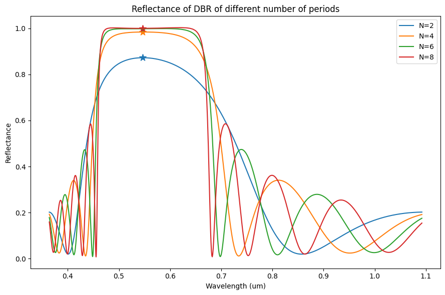
Modify the first activity to calculate the reflectance of DBR devices for N = [2, 4, 6, 8] layers and compare the simulated and analytical results.
We will start by defining a function to create the DBR structure based on the number of pairs.
def build_DBR(N):
    # N is the number of repeated pairs of low/high refractive index material.

    z_0 = 0  # z coordinate of the layer (modify as needed).
    inf_eff = 10  # effective infinity in this model.

    DBR = []  # holder for the DBR structure.

    # build the substrate structure.
    sub = td.Structure(
        geometry=td.Box.from_bounds(
            rmin=(-inf_eff, -inf_eff, -inf_eff), rmax=(inf_eff, inf_eff, 0)
        ),
        medium=medium_s,
    )
    DBR.append(sub)

    # build the first layer.
    layer_1 = td.Structure(
        geometry=td.Box.from_bounds(rmin=(-inf_eff, -inf_eff, 0), rmax=(inf_eff, inf_eff, t_2)),
        medium=medium_2,
    )
    DBR.append(layer_1)
    z_0 = t_2

    # include the N pairs of layers alternatively.
    for i in range(2 * N):
        if i % 2 == 0:
            DBR.append(
                td.Structure(
                    geometry=td.Box.from_bounds(
                        rmin=(-inf_eff, -inf_eff, z_0),
                        rmax=(inf_eff, inf_eff, z_0 + t_1),
                    ),
                    medium=medium_1,
                )
            )
            z_0 = z_0 + t_1
        else:
            DBR.append(
                td.Structure(
                    geometry=td.Box.from_bounds(
                        rmin=(-inf_eff, -inf_eff, z_0),
                        rmax=(inf_eff, inf_eff, z_0 + t_2),
                    ),
                    medium=medium_2,
                )
            )
            z_0 = z_0 + t_2

    return DBR
We will define another function to build the simulation.
def make_DBR(N):

    # build the DBR layers using the previously defined function
    DBR = build_DBR(N)

    thickness = t_2 + N * (t_1 + t_2)  # MODIFY this value to include the DBR multilayer thickness.
    src_z_pos = thickness + lda0 / 4  # source position.
    freq0 = td.C_0 / lda0  # source frequency.
    fwidth = 0.5 * freq0  # width of the frequency distribution.

    plane_wave = td.PlaneWave(
        source_time=td.GaussianPulse(freq0=freq0, fwidth=fwidth),
        size=(td.inf, td.inf, 0),
        center=(0, 0, src_z_pos),
        direction="-",
        pol_angle=0,
    )

    freqs = freq0 * np.linspace(0.5, 1.5, 1001)  # frequency range of interest.

    # Flux monitor to measure the reflectance.
    flux_monitor = td.FluxMonitor(
        center=(0, 0, src_z_pos + lda0 / 4),
        size=(td.inf, td.inf, 0),
        freqs=freqs,
        name="R",
    )

    # Field monitor to visualize the EM field distribution.
    field_xz = td.FieldMonitor(
        center=(0, 0, 0),
        size=(td.inf, 0, td.inf),
        freqs=[freq0],
        name="field_xz",
    )

    Lz = thickness + 2 * lda0  # Domain size in z-direction.

    sim = td.Simulation(
        size=(0, 0, Lz),  # simulation domain size.
        center=(0, 0, thickness / 2),
        grid_spec=td.GridSpec.auto(min_steps_per_wvl=60, wavelength=lda0),
        structures=DBR,
        sources=[plane_wave],
        monitors=[flux_monitor, field_xz],
        run_time=1e-12,
        boundary_spec=td.BoundarySpec(
            x=td.Boundary.periodic(), y=td.Boundary.periodic(), z=td.Boundary.pml()
        ),  # pml is applied in the z-direction.
        shutoff=1e-7,
    )  # early shutoff level is decreased to 1e-7 to increase the simulation accuracy.

    return sim
Then, run a parameter sweep using a Batch object to submit and run all the simulations at once.
Ns = np.array([2, 4, 6, 8])  # collection of N for the parameter sweep.
sims = {f"N={N:.2f}": make_DBR(N) for N in Ns}  # construct simulations for each N from Ns.

# Batch simulation.
batch = web.Batch(simulations=sims, verbose=True)
batch_results = batch.run(path_dir="data")
15:40:39 -03 Created task 'N=2.00' with task_id
             'fdve-c557cd06-209d-45fc-9f54-863bff55b33a' and task_type 'FDTD'.
             View task using web UI at
             'https://tidy3d.simulation.cloud/workbench?taskId=fdve-c557cd06-209
             d-45fc-9f54-863bff55b33a'.
15:40:40 -03 Created task 'N=4.00' with task_id
             'fdve-0774499b-604a-426f-9643-25d0f6167e74' and task_type 'FDTD'.
             View task using web UI at
             'https://tidy3d.simulation.cloud/workbench?taskId=fdve-0774499b-604
             a-426f-9643-25d0f6167e74'.
15:40:42 -03 Created task 'N=6.00' with task_id
             'fdve-cc9eb736-d818-4b18-9f11-13225e5246cc' and task_type 'FDTD'.
             View task using web UI at
             'https://tidy3d.simulation.cloud/workbench?taskId=fdve-cc9eb736-d81
             8-4b18-9f11-13225e5246cc'.
15:40:43 -03 Created task 'N=8.00' with task_id
             'fdve-85ee1ae1-33ac-407f-8ab7-c33b83ce88c2' and task_type 'FDTD'.
             View task using web UI at
             'https://tidy3d.simulation.cloud/workbench?taskId=fdve-85ee1ae1-33a
             c-407f-8ab7-c33b83ce88c2'.
15:40:48 -03 Started working on Batch.
15:40:52 -03 Maximum FlexCredit cost: 0.100 for the whole batch.
             Use 'Batch.real_cost()' to get the billed FlexCredit cost after the
             Batch has completed.
15:41:13 -03 Batch complete.
Finally, we get the simulation results and calculate the analytical reflectance values.
f, ax = plt.subplots(1, 1, figsize=(9, 6), tight_layout=True)

for i, N in enumerate(Ns):
    sim_data = batch_results[f"N={N:.2f}"]
    R = sim_data["R"].flux  # extract reflectance data from the flux monitor
    R_c = (
        ((n_s * n_0 * n_1 ** (2 * N)) - (n_2 ** (2 * N + 2)))
        / ((n_s * n_0 * n_1 ** (2 * N)) + (n_2 ** (2 * N + 2)))
    ) ** 2
    ax.plot(wl_range, R, label=f"N={N}")
    ax.scatter(lda0, R_c, marker="*", s=100)

ax.set_title("Reflectance of DBR of different number of periods")
ax.set_xlabel("Wavelength (um)")
ax.set_ylabel("Reflectance")
ax.legend()
plt.show()
15:41:36 -03 loading simulation from
             data/fdve-c557cd06-209d-45fc-9f54-863bff55b33a.hdf5
15:41:38 -03 loading simulation from
             data/fdve-0774499b-604a-426f-9643-25d0f6167e74.hdf5
15:41:41 -03 loading simulation from
             data/fdve-cc9eb736-d818-4b18-9f11-13225e5246cc.hdf5
15:41:43 -03 loading simulation from
             data/fdve-85ee1ae1-33ac-407f-8ab7-c33b83ce88c2.hdf5
References
[1] Born M, Wolf E, Bhatia AB, et al. Principles of Optics: Electromagnetic Theory of Propagation, Interference and Diffraction of Light. 7th ed. Cambridge: Cambridge University Press; 1999. doi:10.1017/CBO9781139644181